Gradient-Based Iterative Reconstruction

The volume is a tensor of parameters. The differentiable forward projector maps it to projections, a loss compares them with the measurement, and a PyTorch optimizer updates the volume. Autograd computes the gradient with the matched adjoint A^T, so no backprojection code is written by hand.

The same loop takes other losses, regularizers, constraints and network parameters. For least squares without extra terms, the cgls() and sirt() solvers converge in fewer iterations.

Objective

For a projector A and measured projections y, the examples minimize the mean squared error over a nonnegative volume x:

\[\hat{x} = \arg\min_{x \ge 0} \tfrac{1}{M} \lVert A x - y \rVert_2^2\]

M is the number of measured values. After each Adam step, x is clamped to zero or more.

2D parallel and fan beam

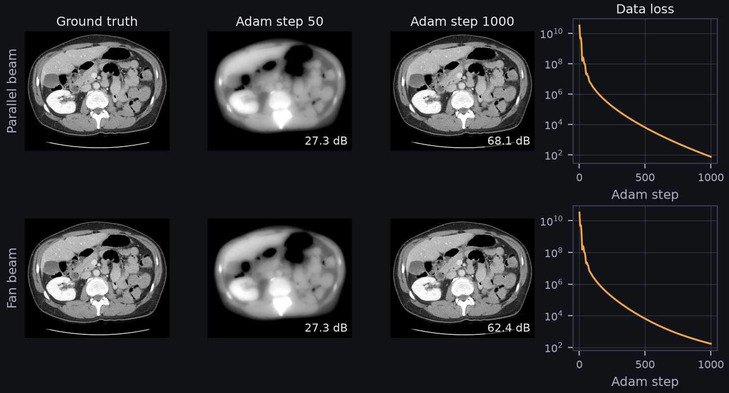
The loop below at 512², with 720 views, Adam learning rate 0.1, 1000 steps and the abdominal slice of TCIA case L213 as ground truth (see Data sources). PSNR uses the peak of the ground truth. The code below uses a 128² square so that it runs in seconds.

Parallel beam

import torch
from diffct import Projector, circular_trajectory_2d_parallel

n, n_views, n_det = 128, 360, 384
trajectory = circular_trajectory_2d_parallel(n_views, device="cuda")
A = Projector(trajectory, (n, n), n_det, beam="parallel", detector_spacing=0.5)

truth = torch.zeros((n, n), device="cuda")
truth[40:88, 40:88] = 1.0
measured = A.project(truth).detach()

image = torch.zeros((n, n), device="cuda", requires_grad=True)
optimizer = torch.optim.Adam([image], lr=0.1)
for step in range(500):
    optimizer.zero_grad()
    loss = 0.5 * (A.project(image) - measured).square().sum()
    loss.backward()
    optimizer.step()
    with torch.no_grad():
        image.clamp_(min=0)

Fan beam

import torch
from diffct import Projector, circular_trajectory_2d_fan

n, n_views = 128, 360
sid, sdd, n_det, pitch = 2.5 * n, 4.0 * n, 3 * n, 0.8
trajectory = circular_trajectory_2d_fan(n_views, sid, sdd, device="cuda")
A = Projector(trajectory, (n, n), n_det, beam="fan", detector_spacing=pitch)

truth = torch.zeros((n, n), device="cuda")
truth[40:88, 40:88] = 1.0
measured = A.project(truth).detach()

image = torch.zeros((n, n), device="cuda", requires_grad=True)
optimizer = torch.optim.Adam([image], lr=0.1)
for step in range(500):
    optimizer.zero_grad()
    loss = 0.5 * (A.project(image) - measured).square().sum()
    loss.backward()
    optimizer.step()
    with torch.no_grad():
        image.clamp_(min=0)

The 2D loops use the summed squared error; its gradient differs from the mean only by a constant factor, and Adam steps are nearly invariant to such a factor.

3D measured walnut

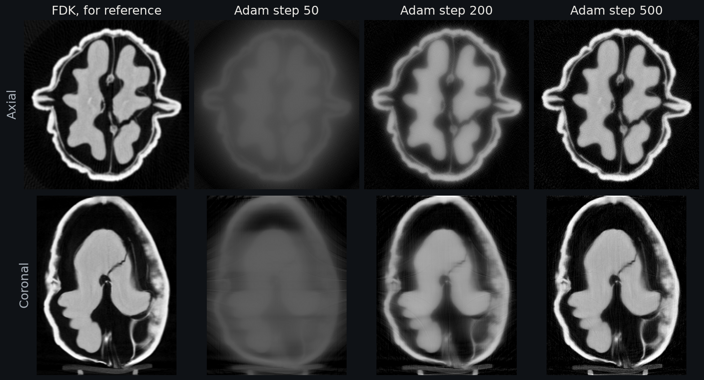
240 measured cone-beam views of a walnut, 256³ volume, Adam with learning rate 0.01. The FDK column is a reference only; the loop starts from zero.

The measured projections are scaled so that the walnut shell is about 1, as in examples/walnut_reconstruction.py:

import torch
from diffct import Projector

# trajectory, detector shape and spacing from examples/walnut_reconstruction.py
A = Projector(trajectory, (256, 256, 256), detector, detector_spacing=(du, dv), voxel_spacing=voxel)

volume = torch.zeros(A.volume_shape, device="cuda", requires_grad=True)
optimizer = torch.optim.Adam([volume], lr=0.01)
for step in range(500):
    optimizer.zero_grad()
    loss = torch.nn.functional.mse_loss(A.project(volume), measured)
    loss.backward()
    optimizer.step()
    with torch.no_grad():
        volume.clamp_(min=0)

The full script is the gradient command of docs/assets/gallery/compute.py.

Variations

• Regularization: add a penalty to the loss, for example loss = loss + weight * diffct.total_variation(volume, voxel_spacing=voxel). tv_reconstruction() packages this loop with residual history and checkpoints.

• Learned components: replace the volume tensor with the output of a network, or make trajectory tensors trainable to calibrate the geometry; see Trajectories and Geometry.

• Large volumes and several GPUs: the same loop works with the devices and distributed options of Projector; see Multiple GPUs and Nodes.

• Stopping: the learning rate and step count are starting values. On real data, stop with a rule that does not use a ground truth.