Differentiable analytical reconstruction

Projector.project and Projector.backproject implement the cell-constant Siddon forward operator and its matched adjoint. Analytical FBP and FDK use a different, voxel-driven interpolation operator. Its backward pass scatters the same interpolation coefficients, including distance weights and normalization. It does not substitute the Siddon projector for the analytical transpose.

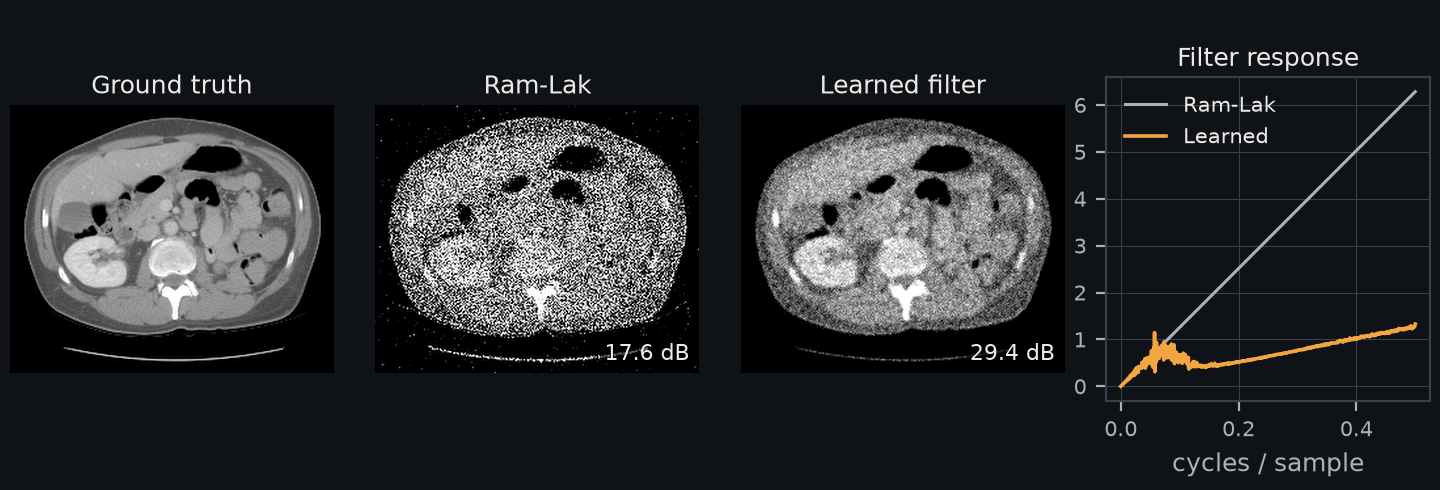
Abdominal slice of TCIA case L213 at 256² (see Data sources), parallel beam, 360 views, 2% noise, 200 Adam steps on the filter only. These settings differ from examples/learnable_reconstruction.py below.

The reconstruction APIs return signed images in the selected precision on the input device. Clamping is a caller decision. In the default native fast mode, low-precision measurements are promoted to float32 before geometry, weighting and FFT operations; gradients retain the original input/parameter dtype. Sinogram, filter and explicit weight gradients propagate through the pipeline, including higher derivatives with respect to those tensors. Acquisition geometry and isocenter are fixed; trainable geometry is rejected explicitly. Use the Siddon Projector for geometry calibration.

Short-scan distance and offset checks account for physical coordinate scale and the original trajectory precision, including when float32 geometry is promoted for float64 measurements. Each check uses only the trajectory components involved in its calculation; detector-v precision cannot relax the detector-u offset check. Each source/detector coordinate and detector-axis component counts with its own rounding along the checked direction, and each allows twice the largest two-view change that this rounding can cause. Axis components have half the smallest subnormal as a rounding floor. Eight eps of the in-plane ray length covers arithmetic and orbit rounding. Both checks also allow a relative tolerance of 1e-4, and the absolute tolerance is at least 1e-5. A change smaller than these bounds cannot be told apart from rounding: low-precision or far-translated coordinates that have a component along the checked direction widen the check. Helical slice centers use float64 independently of the angle dtype; low-precision angles do not round physical voxel coordinates.

fbp and fdk support flat detectors, portable FP32/FP64 arithmetic, view/spatial chunks, several local devices, distributed views/space/hybrid ownership and numerical fbp_into/fdk_into stores; see Precision, training and reconstruction. The helical approximation and low-level CUDA helpers retain their original execution contracts. FDK is an approximate inverse even though its implemented discrete backward pass transposes the interpolation coefficients.

Use the complete APIs with the same trajectory tensors as Projector:

from diffct import fbp, fdk, helical_fdk

image = fbp(sino2d, trajectory2d, (H, W), angles,
            beam="fan", detector_spacing=du, isocenter=(0, 0))
volume = fdk(sino3d, trajectory3d, (D, H, W), angles,
             detector_spacing=(du, dv), isocenter=(0, 0, 0))
helical = helical_fdk(sino3d, helix, (D, H, W), unwrapped_angles,
                      detector_spacing=(du, dv), isocenter=(0, 0, 0))

Sinograms use (views,U) or (views,U,V); images use (H,W) or (D,H,W). Distances, pitches and isocenter share one physical unit. projection_weights replaces the complete pre-filter cosine weight; angular_weights replaces angular quadrature in fbp/fdk. filter_response replaces the full real rFFT multiplier, already scaled in physical units, with length pad_factor*U//2+1. It overrides window. For circular fan/cone short scans, short_scan=True adds Parker weighting before filtering and checks the circular orbit and required angular span. Native curved data needs covered flat-detector resampling before these APIs.

Building and learning a pipeline

Run the examples from a source checkout:

python examples/analytical_reconstruction.py --size 64
python examples/learnable_reconstruction.py --beam parallel --size 32
python examples/learnable_reconstruction.py --beam fan --size 32
python examples/learnable_reconstruction.py --beam cone --size 32
python examples/helical_fdk.py --size 32

learnable_reconstruction.py shows the full pipeline in ordinary PyTorch: detector cosine weights, a trainable frequency response, FFT filtering, angular quadrature and the analytical gather. It optimizes the filter and projection weights for FBP or FDK on a synthetic noisy phantom. This demonstrates autograd and composition; the fitted parameters are specific to the example.

Helical approximation

helical_fdk filters detector rows once, then reconstructs each axial slice from a full turn centered at the angle where the source crosses that slice. helical_view_weights exposes those per-slice quadrature weights. helical_weighted_backproject accepts replacement weights after filtering, so users can learn or replace this stage independently.

This is a native flat-detector, slice-windowed FDK approximation for an axial helix with radial detector normals. It is not an implementation of exact Katsevich inversion, cone-parallel rebinning or conjugate-ray 3D weighting. The source-z samples and explicit unwrapped angles determine the window; nominal pitch parameters are not substituted for the actual acquisition. Incomplete angular windows are rejected. Detector truncation remains possible and the example uses a detector tall enough to cover its selected windows.

The full-turn window and half redundancy factor are motivated by equation 14 of Kong et al. (2018). That paper derives the formula after cone-parallel rebinning; applying the window directly to the native cone gather here is an approximation. Increasing pitch or cone angle can increase reconstruction error.

The implementation processes one slice at a time, keeping the window stage readable and avoiding a views-by-volume weight tensor. This trades kernel-launch overhead for bounded temporary storage; inputs, outputs and autograd state still reside on the CUDA device.

Example results

The 32-voxel learning examples use 180 views and 20 Adam steps on a synthetic phantom with Gaussian projection noise. These training results are specific to that example:

Beam	Initial PSNR	Learned filter/weight PSNR
Parallel FBP	31.96 dB	33.81 dB
Fan FBP	29.90 dB	32.86 dB
Cone FDK	30.24 dB	32.09 dB

The 32-cubed, 720-view, four-turn helical example gives 32.99 dB. The integration weights of each slice sum to pi. Manual composition and the complete API agree within 4e-7. Float32 atomic accumulation order depends on the GPU, so the last digit of these values can change.